Introduction to Scientific Computing

Learning outcome

After the course, the students can evaluate the advantages and disadvantages of graphical and command-line user interfaces and choose the optimal solution for specific tasks. They can use Unix-style operating systems through the command-line interface for basic tasks and automate repetitive tasks using bash scripting. They can utilise Linux services provided by University of Helsinki and CSC – IT Center for Science and can find instructions for using bash scripting on Windows and MacOS computers. From these options, the student can choose the most suitable approach and apply the learned skill in their everyday computing needs.

Motivation

Biosciences have become a data-based discipline, and processing and analysis of large quantities of data is increasingly important. This course provides an accessible introduction to scientific computing through self-learning. The course is a pre-requisite for some computational courses, but the computational skills learned are generic and the course should work as a tutorial to scientific computing methods for students not planning to take those courses. For anyone using computers for data processing, the course hopefully gives ideas on how to efficiently utilise the methods and tools in hand.

One of the primary aims of the course is to provide an easy start for scientific computing and encourage everyone to apply the learned skills in their everyday computer usage. The course uses Linux through a web browser. The University of Helsinki students and staff can keep using the same Linux resources in their studies and work after the completion of this course. The methods learned on this course can naturally be used on one’s own Linux computer; however, they also work on MacOS (which is a Unix-system) and, as a sign of its importance, one can nowadays install and use Linux on Windows computers.

Format

Each chapter starts with a Learning outcome and ends with a Take-home message, clearly visible in framed boxes.

In addition to these, the text contains distinct boxes with additional details or important information. The boxes are collapsed by default and can be opened by clicking the title line.

Some additional information hidden inside

What is a scripting language?

Scripting languages are often considered glue languages that connect different software components or programs. We use scripting in that role and create “wrapper” programs for existing “classical” programs; we also use scripts to manipulate data files before or after they are utilised by more complex programs.

Second, a scripting language has to be easy to write and understand. “Java” and “Python” are two relatively popular and widely-used computer programming languages. Using Java, the text Hello World can be written on the computer screen like this:

public class HelloWorld {
    public void printHelloWorld() {
        System.out.println("Hello World");
    }
    public static void main(String[] args) {
        printHelloWorld();
    }
}

and with Python like this:

print("Hello World")

Of these, Python is considered a scripting language, Java is not.

The self-learning material is accompanied with exercises in Moodle. These exercises are indicated with purple boxes like this:

Exercise: Exercise of something cool..

The exercise would appear here. It would typically start with an explanation of the topic (that should help to complete it) and then have a link to Moodle where the actual exercise is given.

So far, we haven’t really learned anything worth testing…

Efficient and reproducible computing

Here, “scientific computing” means efficient and reproducible use of computers for processing and analysis of data. This could be done with many different operating systems, but Unix is exceptionally well suited for the task and Linux, one variant of that, is used here. As explained elsewhere, most methods learned in this course can also be used on MacOS and Windows systems.

Why should one do this course and learn “scientific computing”:

Automation of repeated tasks. Computers are very good at doing exactly the same task or operation again and again. If a specific task has to be performed once or twice, it may be easier and faster to do it using a program with a graphical user interface (such as Corel Draw, Microsoft Excel); however, if the same task has to be replicated tens, hundreds or thousands of times, it makes sense to write instructions (often called a “script”) for a computer do it. If the instructions are well written, the computer will never make any typos or errors and guarantees to make the task exactly correct every single time.
Reproducible research. The scientific community has started to realise the importance of reproducibility, and an accurate description of the analysis steps is often the requirement for the publication of the findings. One may be able to describe the data processing steps done manually (e.g. “The data was opened in Excel and all rows that contained no data (i.e., the cell content was”NA”) at the fifth column were removed…“), but typically it is easier to describe the processing steps that were done computationally. If other scientists have the same input data and the same programs (more precisely, the same versions of the same programs!), they are guaranteed to get exactly the same output.

In science, the combined impact of these two can be large. First, automation of data processing and analysis (all the way to the production of publication-ready figures!) lowers the bar to re-analyse the data with new observations or new hypotheses – and, in the end, leads to better science. Second, a side effect of utilising computational data processing for reproducible research is that the processing steps become more objective and rule-based than in manual analysis – again, leading to better science.

Surprisingly many computer tasks can be automated relatively easily. The main challenge is to change one’s attitude towards computers: many of us see computers only as a platform where we can do things; this course teaches how we, humans, command the computers to do things for us.

Automation of repetitive tasks: An example of photo editing

Even if you don’t aim to do computer programming and don’t have massive data sets, you may still have good reasons to be interested in the concepts learned on this course. The tricks learned may be useful in your everyday usage of computers. Below is a hypothetical example of a computational task that can be automated. Don’t worry if the details look complex: The point is just to demonstrate the power of automating computational tasks.

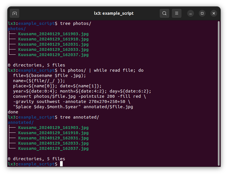
As an example of a task, let’s assume that one has lots of photos with file names indicating the place and time of each photo, e.g. the photo Kuusamo_20240129_161903.jpg was taken in Kuusamo on 29 January 2024 at 16:19:03. For some reason, one would like to have the place and date to be printed in the photo in the format “<place> <date>”. For a small number of photos, this could be done manually with a graphics program (Corel, Adobe, Inkscape etc.); for a larger number of photos this would be quite an effort and it would make sense to automate the task.

In this case, we have six photos:

photos/
├── Helsinki_20240227_164741.jpg
├── Helsinki_20240227_164744.jpg
├── Helsinki_20240227_164746.jpg
├── Kuusamo_20240129_162031.jpg
├── Kuusamo_20240129_162033.jpg
└── Kuusamo_20240129_162037.jpg

and they look like this:

Below is a bash script that loops over the photos, picks up the desired information from the file name, and then uses ImageMagick tool convert to create new photos with the text added at the top.

$ ls photos/ | while read file; do 
  file=$(basename $file .jpg); 
  name=(${file//_/ }); 
  place=${name[0]}; date=${name[1]};
  year=${date:0:4}; month=${date:4:2}; day=${date:6:2};
  convert photos/$file.jpg -pointsize 300 -fill red \
  -gravity southwest -annotate 270x270+750+250 \
  "$place\n$day.$month.$year" annotated/$file.jpg
done

As a result, we have six photos:

annotated/
├── Helsinki_20240227_164741.jpg
├── Helsinki_20240227_164744.jpg
├── Helsinki_20240227_164746.jpg
├── Kuusamo_20240129_162031.jpg
├── Kuusamo_20240129_162033.jpg
└── Kuusamo_20240129_162037.jpg

and they look like this:

These are high-resolution photos (4080x3060 pixels) and running the script took a surprisingly long time, in total 2.8 seconds. Nevertheless, it could be easily applied to hundreds of photos on a regular laptop. I’m a relatively experienced Linux user but had not done this before: I knew that ImageMagick could do it and it took me maybe 20-30 minutes to write the script and create this example (including the shooting of the great photos!). For just six photos, I would have done this task much faster manually using a graphics program; however, now I could do it practically in no time for many more photos. Furthermore, if I would now like to modify the annotation (e.g. change the font size or colour of the text, or add the time of the photo), those changes could be done in a few minutes and then applied to all photos in seconds.

This kind of data processing is also fully reproducible: if I shared the original photos, anyone with ImageMagick could regenerate the same annotated photos. Note that the script may not be fully generic and reproducing the same processing on another set of photos could require some modifications in the convert command. For some reason, ImageMagick thinks that my photos are in landscape and I needed to rotate the annotation text by 270 degrees and place it in the bottom-left corner (i.e., “southwest”). Nevertheless, the script would be a good starting point for doing similar manipulations on other sets of photos.

A good starting point is that most computational tasks can be automated. The main challenge is in finding the right tools for each task! ImageMagick is an amazing program for image editing and processing and it works on all major operating systems. You can find more information about it at https://imagemagick.org/.

Unix and Linux

Unix is a computer operating system (OS) originally developed in the 1970s. Although other OSes became popular on personal computers, Unix remained the backbone of large computing infrastructures. At that time, computers and software were expensive and, as a commercial OS for large companies, Unix was not easily available for hobbyists and computer enthusiasts. In 1991, a student from the University of Helsinki, Linus Torvalds, released Linux, a free Unix-like OS, that could run on a regular personal computer. More specifically, Linux was only the kernel, the engine of the OS, and the functional Linux operating system relied (and still relies) on tools developed by the GNU project.

Nowadays, Linux is by far the most widely used operating system in the world. Windows is more popular on personal computers (PCs), but a version of Linux is found in numerous mobile phones (e.g, all Android phones) and “clever” household appliances (e.g. TV sets, washing machines, fridges). Linux is extremely versatile and scales from simple e-readers to heavy-weight supercomputers. On the most recent list of the world’s 500 most powerful supercomputers, every single one was running Linux. In 2000, Apple released its own Unix-like OS called Darwin that then became the core of MacOS. Since 2016, Microsoft has provided a Windows Subsystem for Linux (WSL) that allows Windows users to run many Linux programs on their Windows computer. (WSL isn’t included in the standard Windows and needs to be installed separately.)

Unix philosophy, shell, terminal and pipes

The design philosophy of Unix was that the OS should provide a set of simple tools, each of which performs a limited and well-defined function, and that these tools can then be freely joined together to form more complex operations and workflows. Below is an example of an analysis workflow where three specialised programs do a specific task one after another. The flows of data from one box to another are called “streams” and the different programs are connected by “pipes”.

  flowchart LR
    A(input) --> B[program_1]
    B --> C[program_2]
    C --> D[program_3]
    D --> E(output)

These tools are controlled with a scripting and command language known as “shell”. The shell commands are given through a computer program called “terminal”.

Linux terminal with bash shell commands.

There are multiple slightly varying shell languages but one of them, known as “bash”, has become dominant and near-standard. Bash is the default shell on Ubuntu (the most popular Linux on personal computers and the one provided by the University of Helsinki) and on old versions of MacOS. (Due to licensing issues, the latest versions of MacOS use the Zsh shell that is largely compatible with Bash.) In this course we use bash.

Simple workflows with “piped” programs are often given as one-line commands in a terminal. More complex workflows (e.g. repetition of specific steps, alternative data flows through tests and conditions) can be written using shell scripts. These can be copy-pasted into a terminal or written to a file that is then executed. In the automation example above, we had a simple structure where a list of items (photos) was piped into a loop that takes the items in order, one item at a time, and performs the specified commands for each of them. Using a pseudo-code, the loop could be described as this:

create_list_of_items | for_each_item_do 
  program_1
  program_2
  program_3
  program_4
until_all_done

Syntax used in the text

The easiest way to learn to use a computer is to use the computer. On this course, you are expected to replicate the commands on a real Linux computer. Those registered for the course get access to the University of Helsinki computer cluster and have the necessary data and programs there. The commands shown should then work by copy-pasting the right text from these instructions into the terminal. The computer commands are shown in distinct boxes like this:

> echo Hello

Hello

Here, the greater-than sign “>” – the first character of the row and separated by a whitespace from everything else – means the command prompt. The prompt may look different on your computer but it typically ends with a greater-than sign or a dollar sign. The actual command is echo Hello and you are supposed to write that in the terminal window (without the proceeding “>”!) and press Enter to execute it; you can also do a copy-paste if the command is long.

The block below (here “Hello”) shows the output of the command.

Command-line prompts

The command-line prompt can vary greatly between systems and, if it is unsatisfactory, one can define its format to own liking. In the Jupyter terminal at CSC it may look like this:

Apptainer> cd ~/IntSciCom/Helsinki/
Apptainer> █

The prompt is fixed and shows always the text Apptainer>. The blinking block is the place where the next command is written.

The Puhti “Login node shell” looks like this:

[username@puhti-login14 ~]$ cd ~/IntSciCom/Helsinki/
[username@puhti-login14 Helsinki]$ █

Here, the first part is the username and, after the @ sign, the name of the computer; the last part inside the square brackets is the current directory. The prompt character is now “$” and the blinking block is for writing the commands.

On my own computer, I have a very minimal prompt:

lx3:~$ cd ~/IntSciCom/Helsinki/
lx3:Helsinki$ █

“lx3” is the name of the computer; I want to know the directory but do not need reminding of my username.

On this course, the command prompt in the examples is >.

Confusingly, both “>” and “$” have other meanings in bash. Typically, “>” doesn’t appear in the beginning of the line and one can distinguish the prompt (which should not copied) and the arrow or greater-than sign from its position. In rare cases, the arrow sign appears as the first character of the command:

> > file.txt

In this case, the first character should be omitted and the actual command is > file.txt. (As we’ll learn later, the arrow directs the contents into a file; as there is nothing on the left side of the arrow, this command empties the file. We’ll come back to this later.)

Sometimes the commands are longer, here consisting of three lines:

> for name in Matti Maija; do
  echo Hello, ${name}!
done

Hello, Matti!
Hello, Maija!

In this case, you should copy-paste (or write) everything from for until done and then press Enter to execute all of it.

If the commands do not produce any visible output and are followed by other commands, the commands should be executed all in row, always excluding the “>” sign. For example, this

> name=Minna
> echo Hello, ${name}!

Hello, Minna!

consists of two commands that both have to be executed to get the final output. An exception to this are the commands like less that are used to browse the data interactively and do not produce a well-defined expected output. In those cases, the output block is not shown.

Later in the course, the output of the commands may be omitted in the instructions and one is expected to make the conclusions from the terminal output.

Different options for doing the course exercises

The whole course can be done on a regular laptop without installation of any new software, using a web browser to connect to the course machine. However, much of the course can be done on a regular laptop without using the remote course machine. If one intends to use the learned skills in everyday work, it makes sense to setup the personal computer such that it can be efficiently used for scientific data analysis. Instructions for setting up a MacOS and Windows system are given in the section Using Bash and command line in everyday work. If in doubt, one may start with the remote machine (explained below) and then later see how to use one’s own computer to do the same. There are a few exercises about the use of the CSC supercomputer that can naturally be performed on CSC computers only.

Options for doing the course exercises:

Own computer: see Using Bash and command line in everyday work, set up the system and come back here.
Remote computer: nevertheless, see Using Bash and command line in everyday work and come back here.

Registration and access to the course machine

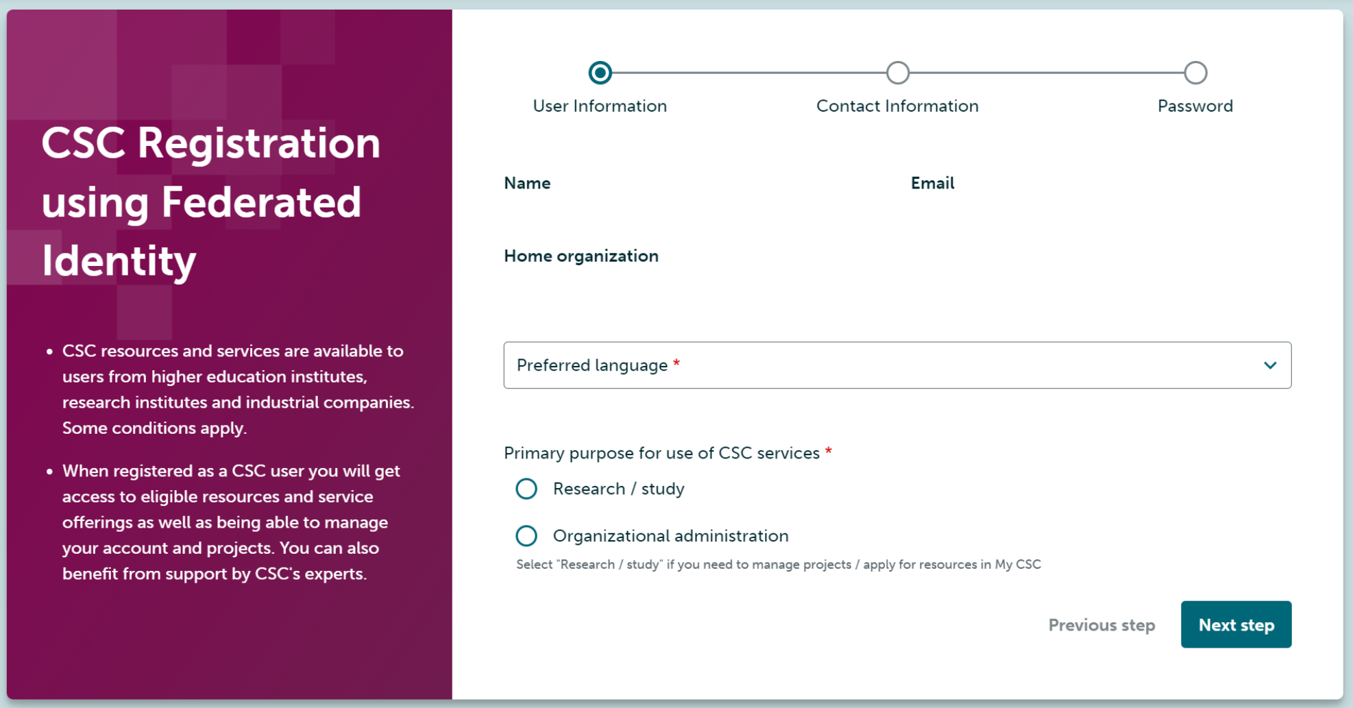
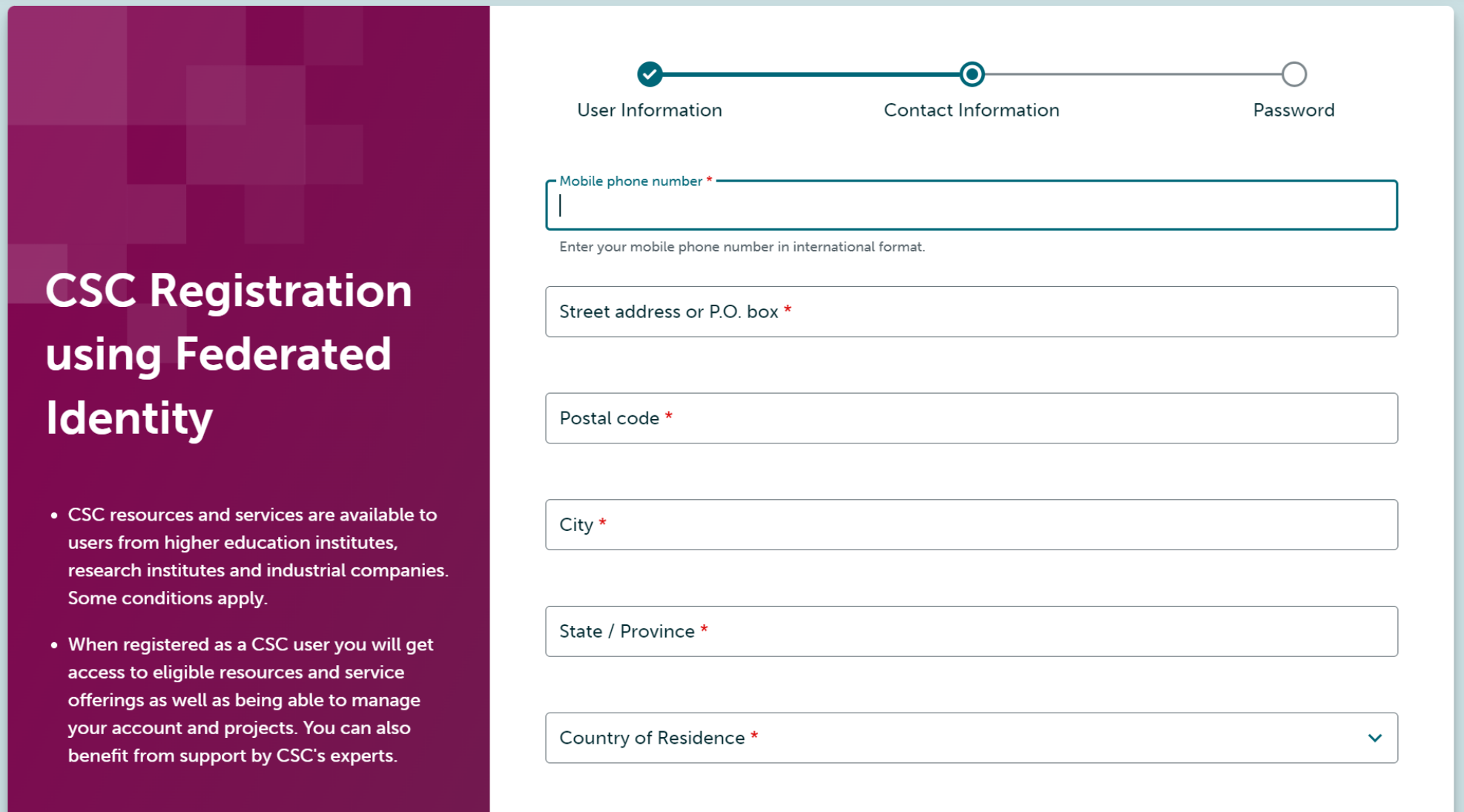
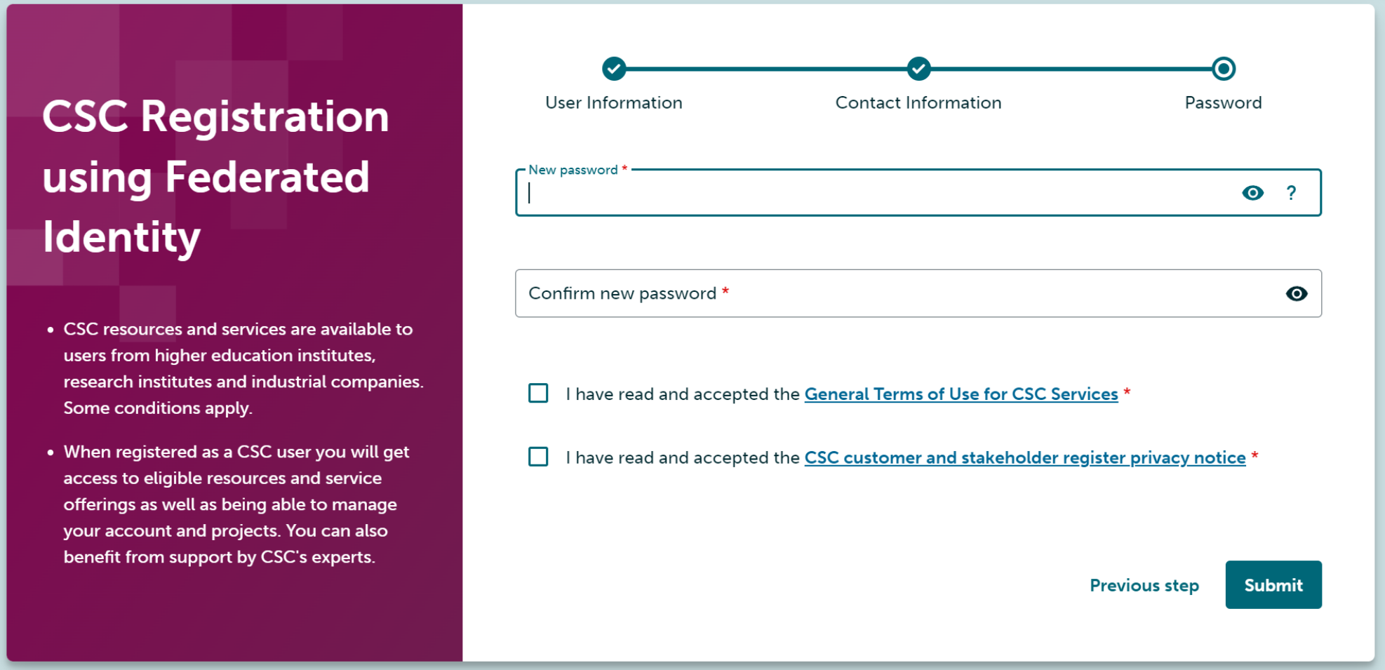
The course material is public and the practicals are designed to be made on the CSC server using the Jupyter interface. The CSC resources are generally available to the university personnel but this course is designed to be performed as a member of a specific CSC project. One can join that CSC group through the link in the Moodle page. The invitation leads to the CSC authentication page:

and selecting “Haka” leads to the UH authentication page. If one doesn’t have an account at CSC, the following pages need to be filled.

Once authenticated, one should apply for membership and wait for the approval. (This is done manually by the teacher and may take some time.)

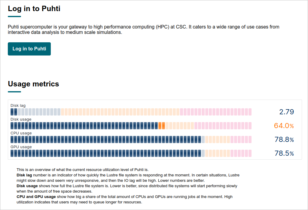
Applying for membership for the course group at CSC.

Once the application has been accepted, one login to the Puhti cluster at https://www.puhti.csc.fi/public/

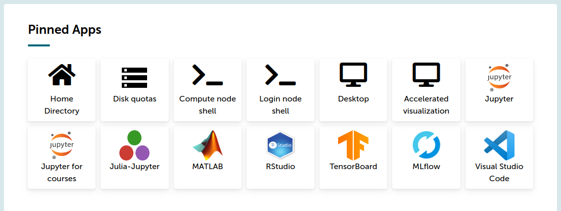
After authenticating (with Haka), one gets to the front page and can click the “Jupyter for Courses” icon (left-bottom):

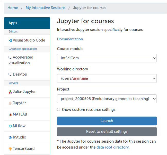
One should confirm that the Course module is “IntSciCom”, the Working directory is one’s home directory (/users/$username) and can then launch the Jupyter tool by clicking the “Launch” button.

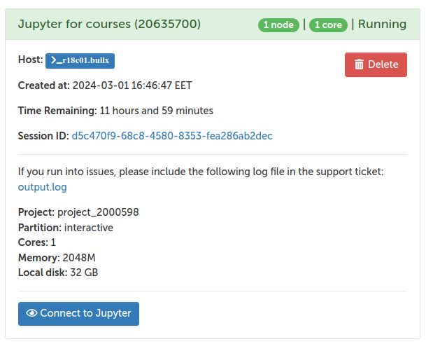
Within one minute, the job at the cluster should be created and the Jupyter screen can be opened by clicking “Connect to Jupyter”:

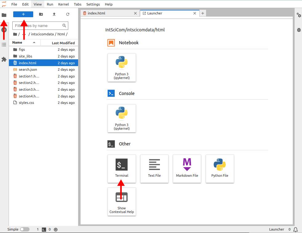
This opens the Jupyter interface and from there one can open a terminal window by clicking the three icons indicated by the red arrows, from left to right:

Here, the text Apptainer > is the prompt after which the commands are written. For example, running the command shown above:

> for name in Matti Maija; do
  echo Hello, ${name}!
done

Hello, Matti!
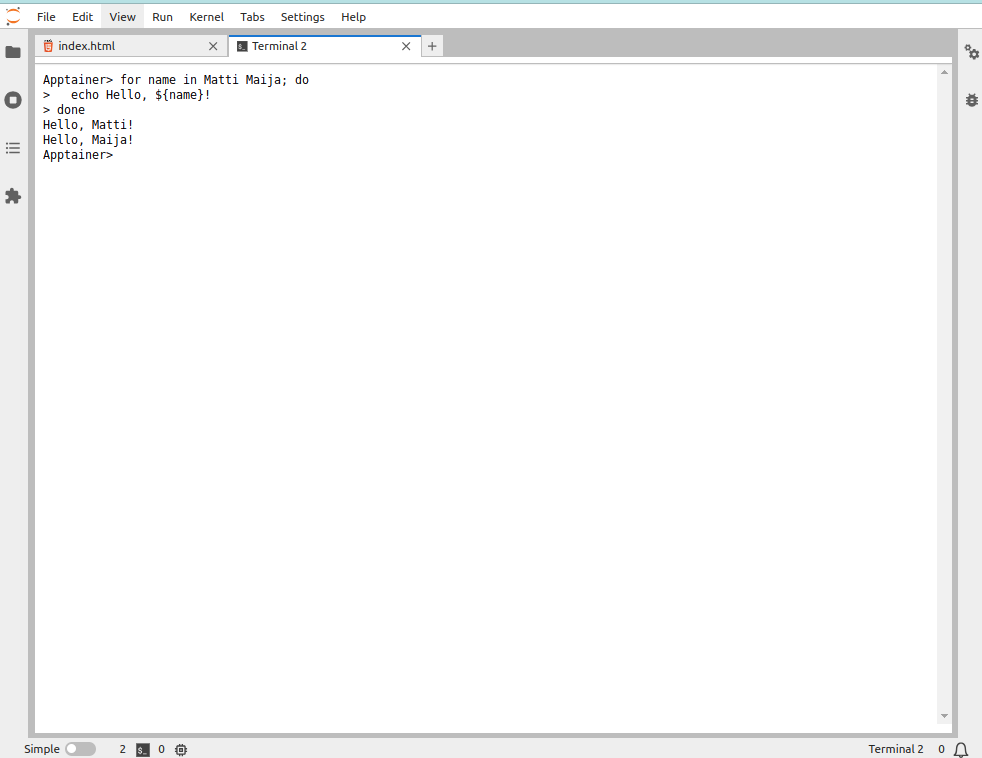
Hello, Maija!

looks like this:

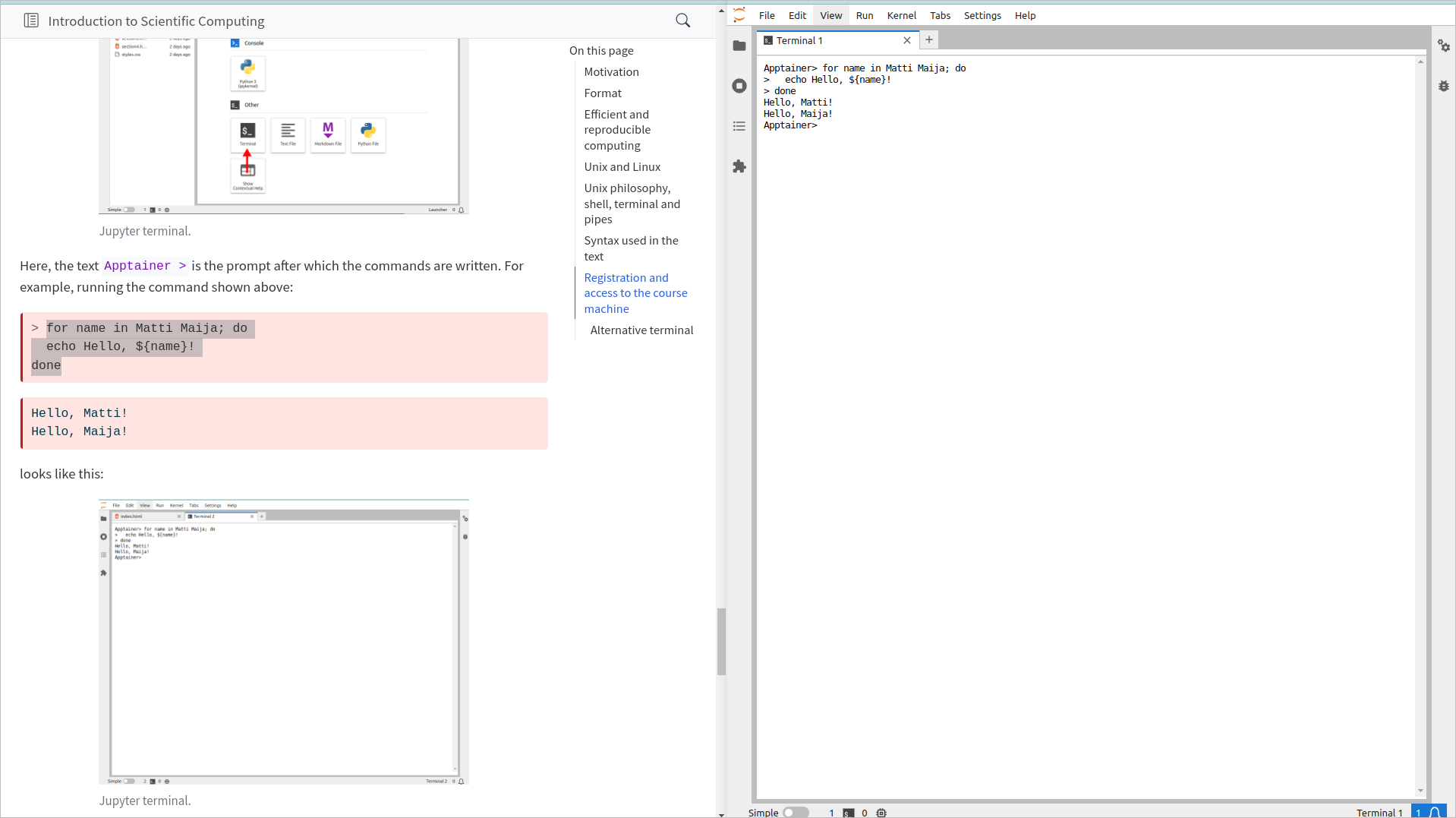
Notice that we copy-pasted the text as is shown above (excluding the “>” in the beginning) and the > signs added at the beginning of each line in the Jupyter terminal output indicate that the same command continues on the next line.

Alternative terminal

The advantage of the Jupyter interface is that it provides a text editor as well as a terminal, and additionally has a file browser to help understanding the directory structure. The downside is that the Jupyter terminal is limited (it lacks a couple of commands used on this course and probably many more that experienced users want to use) and won’t scale for advanced usage. The alternatives are stand-alone terminal programs and connecting to Puhti by SSH (we’ll look at that later) or using the web-based shell program.

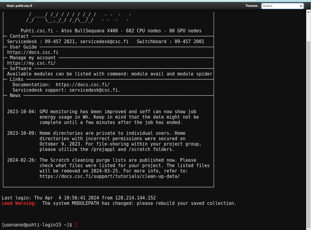
The latter is shown in the front page:

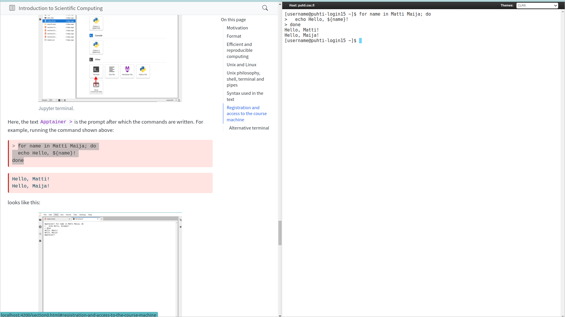
Clicking the “Login node shell” icon opens a new browser window. The default theme is black:

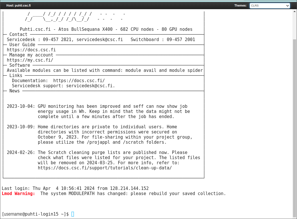
but the colour theme can be changed from the menu in the top-right corner:

Login node shell at Puhti with CLRS colours

I would personally arrange the browser windows such that I could read the documentation on one side and execute the commands on the other side. This can be done with the “Login node shell”:

Recommended arrangement of documentation and terminal

or with the Jupyter terminal:

The third (and best) option is to use a real terminal program to access the CSC machines. That is explained in the section Using Bash and command line in everyday work.

Exercise: Successful login to the CSC Jupyter interface

> cd
> pwd

What is the output of these?

Take-home message

Computers are a great platform to do things – e.g. write texts, draw images or calculate on numbers. The aim of this course is to teach how one can command the computers to do things for us. For that, we will use the command-line interface and the bash scripting language.